Imaging and color measurement · Studies
What do a camera’s spectral sensitivities say about its color fidelity?
A camera does not record color directly. Its red, green, and blue channels each respond to a broad range of wavelengths, and many different spectra can produce the same three channel values. A 3×3 color matrix can align those responses with standard color coordinates, but it cannot recover distinctions that the sensor never recorded.
This study uses retained spectral-sensitivity measurements to ask three questions. Can the sensitivities predict a separately captured color chart? How closely does their three-dimensional subspace approach the CIE standard observer? And after fitting the best linear color transform, how much chart error remains?
Across five measured sensitivity sets the ISO 17321-style index ranges from 88.3 to 90.7 on the 18 chromatic patches, and four of the cameras predicted their paired 140-patch captures to 9.5–13.8% RMS per channel. The fifth has no paired capture, so its closure cells stay empty rather than being filled by inference.
Detailed report · Method and formulas · Published aggregate · Validation controls · Reference code
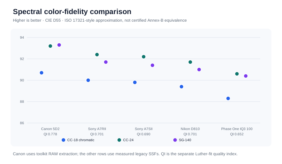
Each group contains three ISO 17321-style sensitivity metamerism index (SMI)
values: the 18 chromatic ColorChecker patches, the full 24-patch chart, and the
140-patch ColorChecker SG. The vertical axis is truncated to 86–94, so it makes
small numeric differences look visually large. The QI label is a separate
Luther-condition quality index; it is not another SMI value. Higher is better
for both indices, but they answer different questions. The footnote records the
sensitivity-source split discussed below: the Canon curves were re-extracted
from RAW, the others are retained measured curves.
Why the archive needs three tests
The retained material is uneven. Four cameras share the laboratory run for which sensitivity curves, a measured illuminant, chart reflectances, and a paired broadband chart capture all survived. Those records permit a physical closure test: predict the chart response from the sensitivities and compare it with what the camera measured.
The Phase One IQ3 sensitivity set came from another rig. It has no paired chart capture in the retained records, so its closure cells are deliberately empty. It can participate in the mathematical sensitivity comparisons, but not in the physical closure experiment.
That separation matters. A good sensitivity-to-observer fit does not prove that the measurement chain predicts a real capture. Conversely, closure residuals include the illuminant, reflectance, capture, and sensitivity records; they are not a pure score of the sensor.
What was calculated
1. Physical closure
For each of the four fully paired camera paths, the measured sensitivities, illuminant, and 140 patch reflectances predict camera RGB. A white-card ratio check runs first. The chart comparison then fits one exposure scale across all patches and all three channels. Separate channel scales would conceal the spectral disagreement the test is intended to expose.
2. Luther-condition quality
The camera’s three sensitivity curves are treated as a vector subspace. Each CIE 1931 color-matching function is fitted from that subspace, and the normalized residuals are combined into a quality index with a ceiling of 1. This isolates the geometric match between the measured sensor and observer subspaces; it does not include a chart, illuminant, exposure, or noise model.
3. ISO 17321-style SMI
The sensitivities synthesize camera RGB for declared reflectance sets under
D55. A 3×3 RGB-to-XYZ matrix is fitted, the remaining CIELAB color differences
are measured, and SMI is calculated as
100 − 5.5 × mean ΔE76. CIEDE2000 is retained as a separate diagnostic. It is
not converted to SMI and is not the same error scale.
Results
| Camera | CC18 SMI | Mean CIEDE2000, CC18 | Luther quality | 140-patch closure RMS by channel |
|---|---|---|---|---|
| Canon 5D2 | 90.7 | 0.93 | 0.778 | 9.539% / 9.840% / 11.618% |
| Sony A7RII | 90.0 | 0.97 | 0.701 | 10.803% / 11.149% / 13.349% |
| Sony A7SII | 89.8 | 0.88 | 0.690 | 9.901% / 9.917% / 11.252% |
| Nikon D810 | 89.4 | 1.07 | 0.701 | 10.802% / 11.069% / 13.802% |
| Phase One IQ3 100 | 88.3 | 1.10 | 0.652 | not available |
Across the five sensitivity sets, CC18 SMI ranges from 88.3 to 90.7 and mean CIEDE2000 spans 0.88 to 1.10 under the declared D55 calculation. No observer experiment or viewing condition in this archive turns the latter range into a universal visibility threshold.
The methods do not produce one interchangeable ranking. The Canon row has the highest CC18 SMI and Luther quality, while the A7SII has the lowest mean CIEDE2000. A7RII and D810 share a Luther quality of 0.701 despite different SMI and CIEDE2000 values. Those differences are useful because they show what each metric responds to; combining them into one score would discard that information.
For the four paired paths, the twelve channel closure residuals span 9.539% to 13.802% RMS. Minimum channel correlation remains above 0.992, but correlation is the weaker result: the 140-patch chart’s large light-to-dark range can preserve ordering even when the response magnitude is wrong. The RMS residual is therefore reported alongside it.
Reference implementation
The relevant calculation from the public C++ implementation.
  // Per-patch raw prediction and the global-scale least-squares fit.
  const std::size_t p = in.patch_ids.size();
  std::array<std::vector<double>, 3> measured, raw_pred;
  for (int c = 0; c < 3; ++c) {
    measured[static_cast<std::size_t>(c)].reserve(p);
    raw_pred[static_cast<std::size_t>(c)].reserve(p);
  }
  double num = 0, den = 0;  // global k = sum(m*pred) / sum(pred*pred)
  for (std::size_t i = 0; i < p; ++i) {
    const auto pred = integrate(in, &in.reflectance[i]);
    for (int c = 0; c < 3; ++c) {
      const double m = in.measured_rgb[i][static_cast<std::size_t>(c)];
      const double pr = pred[static_cast<std::size_t>(c)];
      if (!std::isfinite(pr)) {
        throw std::runtime_error(
            "spectral closure: patch prediction is not representable");
      }
      measured[static_cast<std::size_t>(c)].push_back(m);
      raw_pred[static_cast<std::size_t>(c)].push_back(pr);
      num += m * pr;
      den += pr * pr;
    }
  }
  if (!(den > kEpsilon) || !std::isfinite(den) || !std::isfinite(num)) {
    throw std::runtime_error(
        "spectral closure: global scale is undefined or not representable");
  }
  res.global_scale_k = num / den;
  if (!std::isfinite(res.global_scale_k)) {
    throw std::runtime_error(
        "spectral closure: global scale is not representable");
  }
code/src/spectral_closure.cpp · lines 157–189
What can and cannot be concluded
Within the shared four-camera run, the Canon sensitivity set is the closest to the observer under the declared Luther and SMI calculations. The Phase One value extends the comparison, but it is a directional cross-rig endpoint, not a controlled fifth-camera ranking. The missing overlap means its difference from the shared run cannot be separated from apparatus, wavelength registration, source, geometry, or processing differences.
Two Phase One sweeps were retained, and the last-place result appears under both. They differ by roughly 0.1 SMI, and the camera stays last under either run by both the Luther and the SMI calculation. That is a two-run spread on one rig: it shows that this result does not depend on selecting one of those two retained sweeps, but it bounds nothing about the offset between the two rigs, which remains the larger unknown. The report’s Phase One addendum sets out which questions those records answer, which one they block, and why the blocked one needs a measurement rather than more analysis.
One asymmetry sits inside the winning row itself. Canon’s sensitivity curves were re-extracted from the monochromator RAW captures by this project’s pipeline, while the other four rows are curves measured and retained at the time — so the top-ranked row reached the table by a different processing path than its comparators. That was checked rather than assumed: extractions run the same way for the other three shared-run cameras preserved the Canon and A7SII endpoints, while the D810/A7RII middle pair remained effectively tied and exchanged places at higher precision. For Canon, the retained channel-by-channel comparison between toolkit and legacy curves reaches a normalized response correlation of 0.9993 or better. These controls reduce the chance that curve selection created the ordering; they do not prove that either curve set is physically correct. The table remains mixed-source, and the report states what that does and does not bound.
The closure result shows the narrower point that the four retained sensitivity/capture chains predict their paired 140-patch responses to the reported residuals under one global scale. It does not establish calibration accuracy, an uncertainty bound, or which input contributes most to the error.
What a stronger experiment would add
The preferred experiment would measure every camera on the same documented monochromator and chart setup, repeat the sensitivity sweeps, monitor the source, record dark and pedestal procedures, verify wavelength and bandwidth, and pair each sensitivity set with the same illuminant, physical chart, and broadband capture. Interleaving repeated measurements would support a within-session uncertainty estimate instead of relying on isolated historical runs.
The incomplete archive still answers useful questions because the missing links are kept visible. It shows both what can be recovered from retained measurements and exactly which new acquisition would turn a directional comparison into a controlled one.
Source file: studies/spectral-sensitivity-and-color-fidelity.md